Fitted values and residuals of a rating curve — fitted.rating

The fitted discharge at each gauging, and the residuals: the gaugings' departures from the curve.

Usage

# S3 method for class 'rating_curve'
fitted(object, ...)

# S3 method for class 'rating_curve'
residuals(object, ..., type = c("difference", "scaled"))

Arguments

object: A rating curve fit.
...: Must be empty.
type: The type of residual: "difference" (the default) or "scaled".

Value

A numeric vector, one value per gauging in object$gaugings.

Details

Residuals are calculated on the scale the model is fitted on: the log scale for rc_powerlaw_log(), and discharge, in cubic meters per second, for every other fit. Nothing is transformed back. The type of residual is one of:

"difference": observed minus fitted, so log(observed) - log(fitted) for rc_powerlaw_log().
"scaled": the difference divided by the standard deviation the fit's variance scheme gives at that stage (also known as Pearson residuals). Use these to check the variance scheme: if it is right, they spread about equally at every stage.

Examples

fit <- rc_powerlaw(discharge, stage, data = thompson, variance = "prop")
head(fitted(fit))
#> [1]  253.9909 1971.7884  429.5610  183.9161 2438.9467 2223.4346
head(residuals(fit))
#> [1] 12.009089 28.211560 21.439035 13.083899  1.053319 66.565409

# the residuals in standard deviations, to check the variance scheme
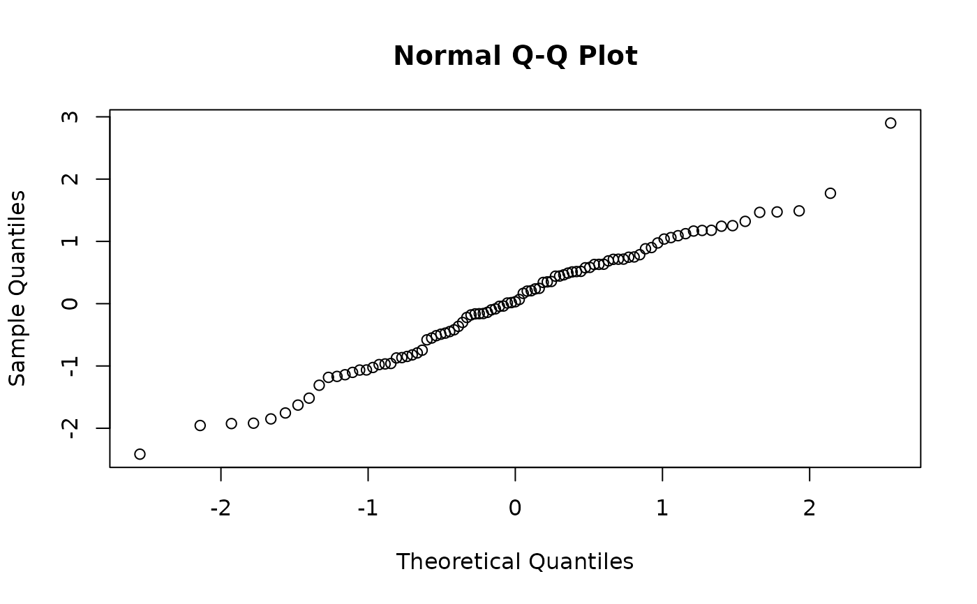
qqnorm(residuals(fit, type = "scaled"))